[ML] 機器學習技法：第六講 Support Vector Regression (SVR)

ML：基礎技法學習
Package：scikit-learn
課程：機器學習技法
簡介：第六講 Support Vector Regression (SVR)

Kernel Ridge Regression (KRR)

$$\begin{array}{rl}\underset{\mathit{\beta }}{min}{E}_{in}(\mathit{\beta })& =\underset{\mathit{\beta }}{min}\frac{\lambda }{N}\sum _{n=1}^N\sum _{m=1}^N{\beta }_n{\beta }_{m}K({\mathbf{x}}_n,{\mathbf{x}}_m)+\frac{1}{N}\sum _{n=1}^N{(y_n-\sum _{m=1}^N{\beta }_{m}K({\mathbf{x}}_n,{\mathbf{x}}_m))}^2\\ & =\underset{\mathit{\beta }}{min}\frac{\lambda }{N}{\mathit{\beta }}^T\mathbf{K}\mathit{\beta }+\frac{1}{N}({\mathit{\beta }}^T{\mathbf{K}}^T\mathbf{K}\mathit{\beta }-2{\mathit{\beta }}^T{\mathbf{K}}^T\mathbf{y}+{\mathbf{y}}^T\mathbf{y})\\ \\ optimal{\mathbf{w}}_{\ast }& =\sum _{n=1}^N{\beta }_n{\mathbf{z}}_n\\ \mathit{\beta }& =(\lambda \mathbf{I}+\mathbf{K}{)}^{-1}\mathbf{y}\end{array}$$ 時間複雜度為 $O(N^3)$，且 $\mathit{\beta }$ 大部分不為 0

L2-regularized linear model
$$\underset{\mathbf{w}}{min}\frac{\lambda }{N}{\mathbf{w}}^T\mathbf{w}+\frac{1}{N}\sum _{n=1}^N(y_n-{\mathbf{w}}^T{\mathbf{z}}_n{)}^2$$ By Representer Theorem optimal ${\mathbf{w}}_{\ast }=\sum _{n=1}^N{\beta }_n{\mathbf{z}}_n$
將 ${\mathbf{w}}_{\ast }$ 代入
$$\begin{array}{rl}\underset{\mathbf{w}}{min}{E}_{in}(\mathbf{w})& =\underset{\mathbf{w}}{min}\frac{\lambda }{N}{\mathbf{w}}^T\mathbf{w}+E_{in}(\mathbf{w})\\ & =\underset{\mathbf{w}}{min}\frac{\lambda }{N}{\mathbf{w}}^T\mathbf{w}+\frac{1}{N}\sum _{n=1}^N(y_n-{\mathbf{w}}^T{\mathbf{z}}_n{)}^2\\ (\because {\mathbf{w}}_{\ast }=\sum _{n=1}^N{\beta }_n{\mathbf{z}}_n=\mathbf{Z}\mathit{\beta })\underset{\mathit{\beta }}{min}{E}_{in}(\mathit{\beta })& =\underset{\mathit{\beta }}{min}\frac{\lambda }{N}(\mathbf{Z}\mathit{\beta }{)}^T\mathbf{Z}\mathit{\beta }+\frac{1}{N}\sum _{n=1}^N(y_n-(\mathbf{Z}\mathit{\beta }{)}^T{\mathbf{z}}_n{)}^2\\ & =\underset{\mathit{\beta }}{min}\frac{\lambda }{N}{\mathit{\beta }}^T{\mathbf{Z}}^T\mathbf{Z}\mathit{\beta }+\frac{1}{N}{\Vert {\mathbf{y}}^T-(\mathbf{Z}\mathit{\beta }{)}^T\mathbf{Z}\Vert }^2\\ & =\underset{\mathit{\beta }}{min}\frac{\lambda }{N}{\mathit{\beta }}^T{\mathbf{Z}}^T\mathbf{Z}\mathit{\beta }+\frac{1}{N}({\mathbf{y}}^T-{\mathit{\beta }}^T{\mathbf{Z}}^T\mathbf{Z})({\mathbf{y}}^T-{\mathit{\beta }}^T{\mathbf{Z}}^T\mathbf{Z}{)}^T\\ & =\underset{\mathit{\beta }}{min}\frac{\lambda }{N}{\mathit{\beta }}^T{\mathbf{Z}}^T\mathbf{Z}\mathit{\beta }+\frac{1}{N}({\mathbf{y}}^T-{\mathit{\beta }}^T{\mathbf{Z}}^T\mathbf{Z})(\mathbf{y}-{\mathbf{Z}}^T\mathbf{Z}\mathit{\beta })\\ & =\underset{\mathit{\beta }}{min}\frac{\lambda }{N}{\mathit{\beta }}^T{\mathbf{Z}}^T\mathbf{Z}\mathit{\beta }+\frac{1}{N}({\mathbf{y}}^T\mathbf{y}-{\mathbf{y}}^T{\mathbf{Z}}^T\mathbf{Z}\mathit{\beta }-{\mathit{\beta }}^T{\mathbf{Z}}^T\mathbf{Z}\mathbf{y}+{\mathit{\beta }}^T{\mathbf{Z}}^T\mathbf{Z}{\mathbf{Z}}^T\mathbf{Z}\mathit{\beta })\\ (\because {\mathbf{Z}}^T\mathbf{Z}=\mathbf{K})& =\underset{\mathit{\beta }}{min}\frac{\lambda }{N}{\mathit{\beta }}^T\mathbf{K}\mathit{\beta }+\frac{1}{N}({\mathbf{y}}^T\mathbf{y}-{\mathbf{y}}^T\mathbf{K}\mathit{\beta }-{\mathit{\beta }}^T\mathbf{K}\mathbf{y}+{\mathit{\beta }}^T\mathbf{K}\mathbf{K}\mathit{\beta })\\ & =\underset{\mathit{\beta }}{min}\frac{\lambda }{N}{\mathit{\beta }}^T\mathbf{K}\mathit{\beta }+\frac{1}{N}({\mathbf{y}}^T\mathbf{y}-{\mathbf{y}}^T\mathbf{K}\mathit{\beta }-{\mathit{\beta }}^T\mathbf{K}\mathbf{y}+{\mathit{\beta }}^T\mathbf{K}\mathbf{K}\mathit{\beta })\\ & =\underset{\mathit{\beta }}{min}\frac{\lambda }{N}{\mathit{\beta }}^T\mathbf{K}\mathit{\beta }+\frac{1}{N}({\mathbf{y}}^T\mathbf{y}-2{\mathit{\beta }}^T\mathbf{K}\mathbf{y}+{\mathit{\beta }}^T\mathbf{K}\mathbf{K}\mathit{\beta })\\ (\because \mathbf{K}issymetric\mathbf{K}={\mathbf{K}}^T)& =\underset{\mathit{\beta }}{min}\frac{\lambda }{N}{\mathit{\beta }}^T\mathbf{K}\mathit{\beta }+\frac{1}{N}({\mathbf{y}}^T\mathbf{y}-2{\mathit{\beta }}^T{\mathbf{K}}^T\mathbf{y}+{\mathit{\beta }}^T{\mathbf{K}}^T\mathbf{K}\mathit{\beta })\\ & =\underset{\mathit{\beta }}{min}\frac{\lambda }{N}{\mathit{\beta }}^T\mathbf{K}\mathit{\beta }+\frac{1}{N}({\mathit{\beta }}^T{\mathbf{K}}^T\mathbf{K}\mathit{\beta }-2{\mathit{\beta }}^T{\mathbf{K}}^T\mathbf{y}+{\mathbf{y}}^T\mathbf{y})\end{array}$$ 若直接展開如下
$$\begin{array}{rl}\underset{\mathbf{w}}{min}{E}_{in}(\mathbf{w})& =\underset{\mathbf{w}}{min}\frac{\lambda }{N}{\mathbf{w}}^T\mathbf{w}+E_{in}(\mathbf{w})\\ & =\underset{\mathbf{w}}{min}\frac{\lambda }{N}{\mathbf{w}}^T\mathbf{w}+\frac{1}{N}\sum _{n=1}^N(y_n-{\mathbf{w}}^T{\mathbf{z}}_n{)}^2\\ (\because {\mathbf{w}}_{\ast }=\sum _{n=1}^N{\beta }_n{\mathbf{z}}_n)\underset{\mathit{\beta }}{min}{E}_{in}(\mathit{\beta })& =\underset{\mathbf{w}}{min}\frac{\lambda }{N}\sum _{n=1}^N{\beta }_n{\mathbf{z}}_n^T\sum _{n=1}^N{\beta }_n{\mathbf{z}}_n+\frac{1}{N}\sum _{n=1}^N(y_n-\sum _{m=1}^N{\beta }_m{\mathbf{z}}_m^T{\mathbf{z}}_n{)}^2\\ & =\underset{\mathbf{w}}{min}\frac{\lambda }{N}\sum _{n=1}^N\sum _{m=1}^N{\beta }_n{\beta }_m{\mathbf{z}}_n^T{\mathbf{z}}_m+\frac{1}{N}\sum _{n=1}^N(y_n-\sum _{m=1}^N{\beta }_m{\mathbf{z}}_m^T{\mathbf{z}}_n{)}^2\\ \because ({\mathbf{z}}_n^T{\mathbf{z}}_m=\mathbf{K}({\mathbf{x}}_n,{\mathbf{x}}_m))& =\underset{\mathbf{w}}{min}\frac{\lambda }{N}\sum _{n=1}^N\sum _{m=1}^N{\beta }_n{\beta }_m\mathbf{K}({\mathbf{x}}_n,{\mathbf{x}}_m)+\frac{1}{N}\sum _{n=1}^N{(y_n-\sum _{m=1}^N{\beta }_m\mathbf{K}({\mathbf{x}}_m,{\mathbf{x}}_n))}^2\\ \because (\mathbf{K}({\mathbf{x}}_m,{\mathbf{x}}_n)=\mathbf{K}({\mathbf{x}}_n,{\mathbf{x}}_m))& =\underset{\mathbf{w}}{min}\frac{\lambda }{N}\sum _{n=1}^N\sum _{m=1}^N{\beta }_n{\beta }_m\mathbf{K}({\mathbf{x}}_n,{\mathbf{x}}_m)+\frac{1}{N}\sum _{n=1}^N{(y_n-\sum _{m=1}^N{\beta }_m\mathbf{K}({\mathbf{x}}_n,{\mathbf{x}}_m))}^2\end{array}$$ 借由矩陣微分
$$\begin{array}{rl}▽E_{in}(\mathit{\beta })& =\frac{\partial }{\partial \mathit{\beta }}(\frac{\lambda }{N}{\mathit{\beta }}^T\mathbf{K}\mathit{\beta }+\frac{1}{N}({\mathit{\beta }}^T{\mathbf{K}}^T\mathbf{K}\mathit{\beta }-2{\mathit{\beta }}^T{\mathbf{K}}^T\mathbf{y}+{\mathbf{y}}^T\mathbf{y}))\\ & =\frac{2\lambda }{N}\mathbf{K}\mathit{\beta }+\frac{1}{N}(2{\mathbf{K}}^T\mathbf{K}\mathit{\beta }-2{\mathbf{K}}^T\mathbf{y})\\ & =\frac{2}{N}(\mathbf{K}\lambda \mathit{\beta }+{\mathbf{K}}^T\mathbf{K}\mathit{\beta }-{\mathbf{K}}^T\mathbf{y})\\ & =\frac{2}{N}{\mathbf{K}}^T(\lambda \mathit{\beta }+\mathbf{K}\mathit{\beta }-\mathbf{y})\\ & =\frac{2}{N}{\mathbf{K}}^T((\lambda \mathbf{I}+\mathbf{K})\mathit{\beta }-\mathbf{y})\end{array}$$ 區域最佳解，微分等於 0，故
$$\begin{array}{rl}▽E_{in}(\mathit{\beta })& =\frac{2}{N}{\mathbf{K}}^T((\lambda \mathbf{I}+\mathbf{K})\mathit{\beta }-\mathbf{y})=0\\ 0& =(\lambda \mathbf{I}+\mathbf{K})\mathit{\beta }-\mathbf{y}\\ \mathit{\beta }& =(\lambda \mathbf{I}+\mathbf{K}{)}^{-1}\mathbf{y}\end{array}$$ 因 $\lambda >0$ 且 $\mathbf{K}$ 為半正定，故反矩陣必定存在
時間複雜度為 $O(N^3)$，且 $\mathit{\beta }$ 大部分不為 0

Support Vector Regression (SVR)

Primal
$$\begin{array}{rl}\underset{\mathbf{b}\mathbf{,}\mathbf{w}\mathbf{,}{\mathit{\xi }}^{\wedge }\mathbf{,}{\mathit{\xi }}^{\vee }}{min}& \frac{1}{2}{\mathbf{w}}^T\mathbf{w}+C\sum _{n=1}^N({\xi }_n^{\wedge }+{\xi }_n^{\vee })\\ s.t.& -ϵ-{\xi }_n^{\vee }\le {\mathbf{w}}^T{\mathbf{z}}_n+b-y_n\le ϵ+{\xi }_n^{\wedge }\\ & {\xi }_n^{\vee }\ge 0,{\xi }_n^{\wedge }\ge 0\end{array}$$ QP of $\tilde{d}+1+N$ 個變數，$2N+2N$ 個條件

Dual
$$\begin{array}{rl}\underset{{\mathit{\alpha }}^{\wedge }\mathbf{,}{\mathit{\alpha }}^{\vee }}{min}& \frac{1}{2}\sum _{n=1}^N\sum _{m=1}^N({\alpha }_n^{\wedge }-{\alpha }_n^{\vee })({\alpha }_m^{\wedge }-{\alpha }_m^{\vee })\mathbf{K}({\mathbf{x}}_n,{\mathbf{x}}_m)+\sum _{n=1}^N((ϵ-y_n){\alpha }_n^{\wedge }+(ϵ+y_n){\alpha }_n^{\vee })\\ s.t.& \sum _{n=1}^N({\alpha }_n^{\wedge }-{\alpha }_n^{\vee })=0\\ & 0\le {\alpha }_n^{\wedge }\le C,0\le {\alpha }_n^{\vee }\le C,\end{array}$$ QP of $2N$ 個變數，$4N+1$ 個條件

$$\begin{gathered} \mathbf{w}=\sum _{n=1}^N\underset{{\beta }_n}{\underbrace{({\alpha }_n^{\wedge }-{\alpha }_n^{\vee })}}{\mathbf{z}}_n \\ C>{\alpha }_n^{\vee }>0 \\ b=y_n-{\mathbf{w}}^T{\mathbf{z}}_n+ϵ \\ C>{\alpha }_n^{\wedge }>0 \\ b=y_n-{\mathbf{w}}^T{\mathbf{z}}_n-ϵ \end{gathered}$$ 只有在 tube 邊界和以外的才是 SV

希望 $\beta$ 的特性與 $\alpha$ 一樣，大部分皆是 0
首先重新定義 err 從 square regression 改為 tube regression

也就是當錯誤在水管範圍內，則視為沒有錯誤，也就是 $|s-y|\le ϵ$ 時，err=0
若超過時，則扣掉水管範圍部分，也就是 $|s-y|>ϵ$ 時，err=$|s-y|-ϵ$
可得 $err(y,s)=max(0,|s-y|-ϵ)$
如圖，可看到 err 在兩者接近 s 時，大約相同，遠離時 tube 成長幅度比較沒那麼劇烈

於是得到 L2-Regularized Tube Regression
$$\underset{\mathbf{w}}{min}\frac{\lambda }{N}{\mathbf{w}}^T\mathbf{w}+\frac{1}{N}\sum _{n=1}^{N}max(0,|{\mathbf{w}}^T{\mathbf{z}}_n-y_n|-ϵ)$$ 為了更接近標準的 SVM 定義，重新調整參數
$$\begin{array}{rl}& \underset{\mathbf{w}}{min}\frac{\lambda }{N}{\mathbf{w}}^T\mathbf{w}+\frac{1}{N}\sum _{n=1}^{N}max(0,|{\mathbf{w}}^T{\mathbf{z}}_n-y_n|-ϵ)\\ \Rightarrow & \underset{\mathbf{w}}{min}\frac{\lambda }{2N}{\mathbf{w}}^T\mathbf{w}+\frac{1}{2N}\sum _{n=1}^{N}max(0,|{\mathbf{w}}^T{\mathbf{z}}_n-y_n|-ϵ)\\ \because \lambda >0\Rightarrow & \underset{\mathbf{w}}{min}\frac{1}{2N}{\mathbf{w}}^T\mathbf{w}+\frac{1}{2N\lambda }\sum _{n=1}^{N}max(0,|{\mathbf{w}}^T{\mathbf{z}}_n-y_n|-ϵ)\\ \because N>0\Rightarrow & \underset{\mathbf{w}}{min}\frac{1}{2}{\mathbf{w}}^T\mathbf{w}+\frac{1}{2\lambda }\sum _{n=1}^{N}max(0,|{\mathbf{w}}^T{\mathbf{z}}_n-y_n|-ϵ)\\ \Rightarrow & \underset{\mathbf{w}}{min}\frac{1}{2}{\mathbf{w}}^T\mathbf{w}+C\sum _{n=1}^{N}max(0,|{\mathbf{w}}^T{\mathbf{z}}_n-y_n|-ϵ)\\ \Rightarrow & \underset{b,\mathbf{w}}{min}\frac{1}{2}{\mathbf{w}}^T\mathbf{w}+C\sum _{n=1}^{N}max(0,|{\mathbf{w}}^T{\mathbf{z}}_n+b-y_n|-ϵ)\end{array}$$ 最後加上 $b$ 的原因，是為了更加符合標準的定義，且因為加上 $b$ 但又對其最小化，不影響原先結果
用 ${\xi }_n$ 表達錯誤，重新定義方程式，當 $|{\mathbf{w}}^T{\mathbf{z}}_n+b-y_n|\le ϵ$ 時，${\xi }_n=0$，不然就 ${\xi }_n>0$
$$\begin{array}{rl}& \underset{b,\mathbf{w}}{min}\frac{1}{2}{\mathbf{w}}^T\mathbf{w}+C\sum _{n=1}^{N}max(0,|{\mathbf{w}}^T{\mathbf{z}}_n+b-y_n|-ϵ)\\ \Rightarrow & \underset{b,\mathbf{w},\mathit{\xi }}{min}\frac{1}{2}{\mathbf{w}}^T\mathbf{w}+C\sum _{n=1}^N{\xi }_n\\ & s.t.|{\mathbf{w}}^T{\mathbf{z}}_n+b-y_n|\le ϵ+{\xi }_n\\ & {\xi }_n\ge 0\end{array}$$ 絕對值仍存在，還不是線性方程式，故再將之展開，並將 ${\xi }_n$ 定義上下限
且將 $|{\mathbf{w}}^T{\mathbf{z}}_n+b-y_n|$ 反向，符合常用定義
$$\begin{array}{rl}& \underset{b,\mathbf{w},\mathit{\xi }}{min}\frac{1}{2}{\mathbf{w}}^T\mathbf{w}+C\sum _{n=1}^N{\xi }_n\\ & s.t.|{\mathbf{w}}^T{\mathbf{z}}_n+b-y_n|\le ϵ+{\xi }_n\\ & {\xi }_n\ge 0\\ \Rightarrow & \underset{b,\mathbf{w},{\mathit{\xi }}^{\vee },{\mathit{\xi }}^{\wedge }}{min}\frac{1}{2}{\mathbf{w}}^T\mathbf{w}+C\sum _{n=1}^N({\xi }_n^{\vee }+{\xi }_n^{\wedge })\\ & s.t.-ϵ-{\xi }_n^{\vee }\le y_n-{\mathbf{w}}^T{\mathbf{z}}_n-b\le ϵ+{\xi }_n^{\wedge }\\ & {\xi }_n^{\vee }\ge 0,{\xi }_n^{\wedge }\ge 0\end{array}$$ 故可得 primal，QP of $\tilde{d}+1+N$ 個變數，$2N+2N$ 個條件

但這還不是想要的，dual 又該如何得到呢？
利用 Lagrange multipliers，隱藏限制條件，此處將 ${\lambda }_n$ 用 ${\alpha }_n^{\wedge }$ & ${\alpha }_n^{\vee }$ & ${\beta }_n^{\wedge }$ & ${\beta }_n^{\vee }$ 取代
$$L(b,\mathbf{w},{\mathit{\xi }}^{\vee },{\mathit{\xi }}^{\wedge },{\mathit{\alpha }}^{\vee },{\mathit{\alpha }}^{\wedge },{\mathit{\beta }}^{\vee },{\mathit{\beta }}^{\wedge })=\frac{1}{2}{\mathbf{w}}^T\mathbf{w}+C\cdot \sum _{n=1}^N({\xi }_n^{\vee }+{\xi }_n^{\wedge })+\sum _{n=1}^N{\alpha }_n^{\vee }(-y_n+{\mathbf{w}}^T{\mathbf{z}}_n+b-ϵ-{\xi }_n^{\vee })+\sum _{n=1}^N{\alpha }_n^{\wedge }(y_n-{\mathbf{w}}^T{\mathbf{z}}_n-b-ϵ-{\xi }_n^{\wedge })+\sum _{n=1}^N{\beta }_n^{\wedge }\cdot (-{\xi }_n^{\wedge })+\sum _{n=1}^N{\beta }_n^{\vee }\cdot (-{\xi }_n^{\vee })$$ 當 $\underset{all{\alpha }_n^{\vee }\ge 0,{\alpha }_n^{\wedge }\ge 0,{\beta }_n^{\vee }\ge 0,{\beta }_n^{\wedge }\ge 0}{max}L(b,\mathbf{w},{\mathit{\xi }}^{\vee },{\mathit{\xi }}^{\wedge },{\mathit{\alpha }}^{\vee },{\mathit{\alpha }}^{\wedge },{\mathit{\beta }}^{\vee },{\mathit{\beta }}^{\wedge })$ 會發現

• $(b,\mathbf{w},{\mathit{\xi }}^{\vee },{\mathit{\xi }}^{\wedge })$ 違反限制條件時，會導致
•  $-y_n+{\mathbf{w}}^T{\mathbf{z}}_n+b-ϵ-{\xi }_n^{\vee }>0$
  又因 $L(b,\mathbf{w},{\mathit{\xi }}^{\vee },{\mathit{\xi }}^{\wedge },{\mathit{\alpha }}^{\vee },{\mathit{\alpha }}^{\wedge },{\mathit{\beta }}^{\vee },{\mathit{\beta }}^{\wedge })$ 針對 ${\alpha }_n^{\vee }$ 取 max 的緣故，${\alpha }_n^{\vee }$ 越大越好
•  $y_n-{\mathbf{w}}^T{\mathbf{z}}_n-b-ϵ-{\xi }_n^{\wedge }>0$
  又因 $L(b,\mathbf{w},{\mathit{\xi }}^{\vee },{\mathit{\xi }}^{\wedge },{\mathit{\alpha }}^{\vee },{\mathit{\alpha }}^{\wedge },{\mathit{\beta }}^{\vee },{\mathit{\beta }}^{\wedge })$ 針對 ${\alpha }_n^{\wedge }$ 取 max 的緣故，${\alpha }_n^{\wedge }$ 越大越好
•  $-{\xi }_n^{\vee }>0$
  又因 $L(b,\mathbf{w},{\mathit{\xi }}^{\vee },{\mathit{\xi }}^{\wedge },{\mathit{\alpha }}^{\vee },{\mathit{\alpha }}^{\wedge },{\mathit{\beta }}^{\vee },{\mathit{\beta }}^{\wedge })$ 針對 ${\beta }_n^{\vee }$ 取 max 的緣故，${\beta }_n^{\vee }$ 越大越好
•  $-{\xi }_n^{\wedge }>0$
  又因 $L(b,\mathbf{w},{\mathit{\xi }}^{\vee },{\mathit{\xi }}^{\wedge },{\mathit{\alpha }}^{\vee },{\mathit{\alpha }}^{\wedge },{\mathit{\beta }}^{\vee },{\mathit{\beta }}^{\wedge })$ 針對 ${\beta }_n^{\wedge }$ 取 max 的緣故，${\beta }_n^{\wedge }$ 越大越好
• 使得 $L(b,\mathbf{w},{\mathit{\xi }}^{\vee },{\mathit{\xi }}^{\wedge },{\mathit{\alpha }}^{\vee },{\mathit{\alpha }}^{\wedge },{\mathit{\beta }}^{\vee },{\mathit{\beta }}^{\wedge })\to \mathrm{\infty }$
• $(b,\mathbf{w},{\mathit{\xi }}^{\vee },{\mathit{\xi }}^{\wedge })$ 符合限制條件時，會導致
• $-y_n+{\mathbf{w}}^T{\mathbf{z}}_n+b-ϵ-{\xi }_n^{\vee }\le 0$
  又因 $L(b,\mathbf{w},{\mathit{\xi }}^{\vee },{\mathit{\xi }}^{\wedge },{\mathit{\alpha }}^{\vee },{\mathit{\alpha }}^{\wedge },{\mathit{\beta }}^{\vee },{\mathit{\beta }}^{\wedge })$ 針對 ${\alpha }_n^{\vee }$ 取 max 的緣故，${\alpha }_n^{\vee }$ 與 $-y_n+{\mathbf{w}}^T{\mathbf{z}}_n+b-ϵ-{\xi }_n^{\vee }$ 兩者至少有一個必須為 0
• $y_n-{\mathbf{w}}^T{\mathbf{z}}_n-b-ϵ-{\xi }_n^{\wedge }\le 0$
  又因 $L(b,\mathbf{w},{\mathit{\xi }}^{\vee },{\mathit{\xi }}^{\wedge },{\mathit{\alpha }}^{\vee },{\mathit{\alpha }}^{\wedge },{\mathit{\beta }}^{\vee },{\mathit{\beta }}^{\wedge })$ 針對 ${\alpha }_n^{\wedge }$ 取 max 的緣故，${\alpha }_n^{\wedge }$ 與 $y_n-{\mathbf{w}}^T{\mathbf{z}}_n-b-ϵ-{\xi }_n^{\wedge }$ 兩者至少有一個必須為 0
•  $-{\xi }_n^{\vee }\le 0$
  又因 $L(b,\mathbf{w},{\mathit{\xi }}^{\vee },{\mathit{\xi }}^{\wedge },{\mathit{\alpha }}^{\vee },{\mathit{\alpha }}^{\wedge },{\mathit{\beta }}^{\vee },{\mathit{\beta }}^{\wedge })$ 針對 ${\beta }_n^{\vee }$ 取 max 的緣故，${\beta }_n^{\vee }$ 與 $-{\xi }_n^{\vee }$ 兩者至少有一個必須為 0
•  $-{\xi }_n^{\wedge }\le 0$
  又因 $L(b,\mathbf{w},{\mathit{\xi }}^{\vee },{\mathit{\xi }}^{\wedge },{\mathit{\alpha }}^{\vee },{\mathit{\alpha }}^{\wedge },{\mathit{\beta }}^{\vee },{\mathit{\beta }}^{\wedge })$ 針對 ${\beta }_n^{\wedge }$ 取 max 的緣故，${\beta }_n^{\wedge }$ 與 $-{\xi }_n^{\wedge }$ 兩者至少有一個必須為 0
• 使得 $L(b,\mathbf{w},{\mathit{\xi }}^{\vee },{\mathit{\xi }}^{\wedge },{\mathit{\alpha }}^{\vee },{\mathit{\alpha }}^{\wedge },{\mathit{\beta }}^{\vee },{\mathit{\beta }}^{\wedge })\to \frac{1}{2}{\mathbf{w}}^T\mathbf{w}$

故此式子與原本的求解一樣，如下，只是限制條件被隱藏到 max 中
$$SVM\equiv \underset{b,\mathbf{w},{\mathit{\xi }}^{\vee },{\mathit{\xi }}^{\wedge }}{min}(\underset{all{\alpha }_n^{\vee }\ge 0,{\alpha }_n^{\wedge }\ge 0,{\beta }_n^{\vee }\ge 0,{\beta }_n^{\wedge }\ge 0}{max}L(b,\mathbf{w},{\mathit{\xi }}^{\vee },{\mathit{\xi }}^{\wedge },{\mathit{\alpha }}^{\vee },{\mathit{\alpha }}^{\wedge },{\mathit{\beta }}^{\vee },{\mathit{\beta }}^{\wedge }))=\underset{b,\mathbf{w},{\mathit{\xi }}^{\vee },{\mathit{\xi }}^{\wedge }}{min}(\mathrm{\infty }ifviolate;\frac{1}{2}{\mathbf{w}}^T\mathbf{w}iffeasible)$$
此時 $(b,\mathbf{w},{\mathit{\xi }}^{\vee },{\mathit{\xi }}^{\wedge })$ 仍在式子最外面，如何把它跟裡面的 ${\alpha }_n^{\wedge },{\alpha }_n^{\vee },{\beta }_n^{\wedge },{\beta }_n^{\vee }$ 交換呢？
這樣才能初步得到 4N 個變數的式子
任取一個 ${\mathit{\alpha }}^{\prime \vee },{\mathit{\alpha }}^{\prime \wedge },{\mathit{\beta }}^{\prime \vee },{\mathit{\beta }}^{\prime \wedge }$ with ${\alpha }_n^{\prime \vee }\ge 0,{\alpha }_n^{\prime \wedge }\ge 0,{\beta }_n^{\prime \vee }\ge 0,{\beta }_n^{\prime \wedge }\ge 0$
因取 max 一定比任意還大，可得下式
$\underset{b,\mathbf{w},{\mathit{\xi }}^{\vee },{\mathit{\xi }}^{\wedge }}{min}(\underset{all{\alpha }_n^{\vee }\ge 0,{\alpha }_n^{\wedge }\ge 0,{\beta }_n^{\vee }\ge 0,{\beta }_n^{\wedge }\ge 0}{max}L(b,\mathbf{w},{\mathit{\xi }}^{\vee },{\mathit{\xi }}^{\wedge },{\mathit{\alpha }}^{\vee },{\mathit{\alpha }}^{\wedge },{\mathit{\beta }}^{\vee },{\mathit{\beta }}^{\wedge }))\ge \underset{b,\mathbf{w},{\mathit{\xi }}^{\vee },{\mathit{\xi }}^{\wedge }}{min}L(b,\mathbf{w},{\mathit{\xi }}^{\vee },{\mathit{\xi }}^{\wedge },{\mathit{\alpha }}^{\prime \vee },{\mathit{\alpha }}^{\prime \wedge },{\mathit{\beta }}^{\prime \vee },{\mathit{\beta }}^{\prime \wedge })$
那如果對 ${\mathit{\alpha }}^{\prime \vee }\ge 0,{\mathit{\alpha }}^{\prime \wedge }\ge 0,{\mathit{\beta }}^{\prime \vee }\ge 0,{\mathit{\beta }}^{\prime \wedge }\ge 0$ 取 max，也不影響此等式，如下
$\underset{b,\mathbf{w},{\mathit{\xi }}^{\vee },{\mathit{\xi }}^{\wedge }}{min}(\underset{all{\alpha }_n^{\vee }\ge 0,{\alpha }_n^{\wedge }\ge 0,{\beta }_n^{\vee }\ge 0,{\beta }_n^{\wedge }\ge 0}{max}L(b,\mathbf{w},{\mathit{\xi }}^{\vee },{\mathit{\xi }}^{\wedge },{\mathit{\alpha }}^{\vee },{\mathit{\alpha }}^{\wedge },{\mathit{\beta }}^{\vee },{\mathit{\beta }}^{\wedge }))\ge \underset{Lagrangedualproblem}{\underbrace{\underset{all{\mathit{\alpha }}^{\prime \vee }\ge 0,{\mathit{\alpha }}^{\prime \wedge }\ge 0,{\mathit{\beta }}^{\prime \vee }\ge 0,{\mathit{\beta }}^{\prime \wedge }\ge 0}{max}(\underset{b,\mathbf{w},{\mathit{\xi }}^{\vee },{\mathit{\xi }}^{\wedge }}{min}L(b,\mathbf{w},{\mathit{\xi }}^{\vee },{\mathit{\xi }}^{\wedge },{\mathit{\alpha }}^{\prime \vee },{\mathit{\alpha }}^{\prime \wedge },{\mathit{\beta }}^{\prime \vee },{\mathit{\beta }}^{\prime \wedge }))\stackrel{{\mathit{\alpha }}^{\prime \vee }={\mathit{\alpha }}^{\vee },{\mathit{\alpha }}^{\prime \wedge }={\mathit{\alpha }}^{\wedge },{\mathit{\beta }}^{\prime \vee }={\mathit{\beta }}^{\vee },{\mathit{\beta }}^{\prime \wedge }={\mathit{\beta }}^{\wedge }}{\to }\underset{all{\alpha }_n^{\vee }\ge 0,{\alpha }_n^{\wedge }\ge 0,{\beta }_n^{\vee }\ge 0,{\beta }_n^{\wedge }\ge 0}{max}(\underset{b,\mathbf{w},{\mathit{\xi }}^{\vee },{\mathit{\xi }}^{\wedge }}{min}L(b,\mathbf{w},{\mathit{\xi }}^{\vee },{\mathit{\xi }}^{\wedge },{\mathit{\alpha }}^{\vee },{\mathit{\alpha }}^{\wedge },{\mathit{\beta }}^{\vee },{\mathit{\beta }}^{\wedge }))}}$
比較直覺的想法，就像是「從最大的一群中取最小」一定 $\ge$ 「從最小的一群中取最大」
$$\underset{original(primal))SVM}{\underbrace{\underset{b,\mathbf{w},{\mathit{\xi }}^{\vee },{\mathit{\xi }}^{\wedge }}{min}(\underset{all{\alpha }_n^{\vee }\ge 0,{\alpha }_n^{\wedge }\ge 0,{\beta }_n^{\vee }\ge 0,{\beta }_n^{\wedge }\ge 0}{max}L(b,\mathbf{w},{\mathit{\xi }}^{\vee },{\mathit{\xi }}^{\wedge },{\mathit{\alpha }}^{\vee },{\mathit{\alpha }}^{\wedge },{\mathit{\beta }}^{\vee },{\mathit{\beta }}^{\wedge }))}}\ge \underset{Lagrangedual}{\underbrace{\underset{all{\alpha }_n^{\vee }\ge 0,{\alpha }_n^{\wedge }\ge 0,{\beta }_n^{\vee }\ge 0,{\beta }_n^{\wedge }\ge 0}{max}(\underset{b,\mathbf{w},{\mathit{\xi }}^{\vee },{\mathit{\xi }}^{\wedge }}{min}L(b,\mathbf{w},{\mathit{\xi }}^{\vee },{\mathit{\xi }}^{\wedge },{\mathit{\alpha }}^{\vee },{\mathit{\alpha }}^{\wedge },{\mathit{\beta }}^{\vee },{\mathit{\beta }}^{\wedge }))}}$$ 目前的關係稱作 $\ge$ weak duality

但這還不夠，最好是 $=$ strong duality，才能初步得到 4N 個變數的式子
幸運的是，在 QP 中，只要滿足以下條件，便是 strong duality

• convex primal (原來的問題為 convex)
• feasible primal (原來的問題有解的，也就是線性可分)
• linear constraints (限制條件為線性的)

對於 SVM 滿足這些條件並不困難，故解以下的式子，如同解原本的式子
$$\underset{all{\alpha }_n^{\vee }\ge 0,{\alpha }_n^{\wedge }\ge 0,{\beta }_n^{\vee }\ge 0,{\beta }_n^{\wedge }\ge 0}{max}\left(\underset{b,\mathbf{w},{\mathit{\xi }}^{\vee },{\mathit{\xi }}^{\wedge }}{min}\underset{L(b,\mathbf{w},{\mathit{\xi }}^{\vee },{\mathit{\xi }}^{\wedge },{\mathit{\alpha }}^{\vee },{\mathit{\alpha }}^{\wedge },{\mathit{\beta }}^{\vee },{\mathit{\beta }}^{\wedge })}{\underbrace{\frac{1}{2}{\mathbf{w}}^T\mathbf{w}+C\cdot \sum _{n=1}^N({\xi }_n^{\vee }+{\xi }_n^{\wedge })+\sum _{n=1}^N{\alpha }_n^{\vee }(-y_n+{\mathbf{w}}^T{\mathbf{z}}_n+b-ϵ-{\xi }_n^{\vee })+\sum _{n=1}^N{\alpha }_n^{\wedge }(y_n-{\mathbf{w}}^T{\mathbf{z}}_n-b-ϵ-{\xi }_n^{\wedge })+\sum _{n=1}^N{\beta }_n^{\wedge }\cdot (-{\xi }_n^{\wedge })+\sum _{n=1}^N{\beta }_n^{\vee }\cdot (-{\xi }_n^{\vee })}}\right)$$
但如何把內部的 $(b,\mathbf{w},{\mathit{\xi }}^{\vee },{\mathit{\xi }}^{\wedge })$ 拿掉呢？
內部的問題，當最佳化時，必定符合
$$\begin{array}{rl}\frac{\partial L(b,\mathbf{w},{\mathit{\xi }}^{\vee },{\mathit{\xi }}^{\wedge },{\mathit{\alpha }}^{\vee },{\mathit{\alpha }}^{\wedge },{\mathit{\beta }}^{\vee },{\mathit{\beta }}^{\wedge })}{\partial b}& =0=\sum _{n=1}^N({\alpha }_n^{\vee }-{\alpha }_n^{\wedge })\Rightarrow \sum _{n=1}^N({\alpha }_n^{\wedge }-{\alpha }_n^{\vee })=0\\ \frac{\partial L(b,\mathbf{w},{\mathit{\xi }}^{\vee },{\mathit{\xi }}^{\wedge },{\mathit{\alpha }}^{\vee },{\mathit{\alpha }}^{\wedge },{\mathit{\beta }}^{\vee },{\mathit{\beta }}^{\wedge })}{\partial \mathbf{w}}& =\mathbf{0}=\mathbf{w}+\sum _{n=1}^N{\alpha }_n^{\vee }{\mathbf{z}}_n-\sum _{n=1}^N{\alpha }_n^{\wedge }{\mathbf{z}}_n\Rightarrow \mathbf{w}=\sum _{n=1}^N\underset{{\beta }_n}{\underbrace{({\alpha }_n^{\wedge }-{\alpha }_n^{\vee })}}{\mathbf{z}}_n\\ \frac{\partial L(b,\mathbf{w},{\mathit{\xi }}^{\vee },{\mathit{\xi }}^{\wedge },{\mathit{\alpha }}^{\vee },{\mathit{\alpha }}^{\wedge },{\mathit{\beta }}^{\vee },{\mathit{\beta }}^{\wedge })}{\partial {\xi }^{\vee }}& =0=C-{\alpha }_n^{\vee }-{\beta }_n^{\vee }\Rightarrow {\beta }_n^{\vee }=C-{\alpha }_n^{\vee }\\ \frac{\partial L(b,\mathbf{w},{\mathit{\xi }}^{\vee },{\mathit{\xi }}^{\wedge },{\mathit{\alpha }}^{\vee },{\mathit{\alpha }}^{\wedge },{\mathit{\beta }}^{\vee },{\mathit{\beta }}^{\wedge })}{\partial {\xi }^{\wedge }}& =0=C-{\alpha }_n^{\wedge }-{\beta }_n^{\wedge }\Rightarrow {\beta }_n^{\wedge }=C-{\alpha }_n^{\wedge }\end{array}$$ 從以上的這些條件，可得
$$\begin{array}{rl}dual& =\underset{all{\alpha }_n^{\vee }\ge 0,{\alpha }_n^{\wedge }\ge 0,{\beta }_n^{\vee }\ge 0,{\beta }_n^{\wedge }\ge 0}{max}(\underset{b,\mathbf{w},{\mathit{\xi }}^{\vee },{\mathit{\xi }}^{\wedge }}{min}\frac{1}{2}{\mathbf{w}}^T\mathbf{w}+C\cdot \sum _{n=1}^N({\xi }_n^{\vee }+{\xi }_n^{\wedge })+\sum _{n=1}^N{\alpha }_n^{\vee }(-y_n+{\mathbf{w}}^T{\mathbf{z}}_n+b-ϵ-{\xi }_n^{\vee })+\sum _{n=1}^N{\alpha }_n^{\wedge }(y_n-{\mathbf{w}}^T{\mathbf{z}}_n-b-ϵ-{\xi }_n^{\wedge })+\sum _{n=1}^N{\beta }_n^{\wedge }\cdot (-{\xi }_n^{\wedge })+\sum _{n=1}^N{\beta }_n^{\vee }\cdot (-{\xi }_n^{\vee }))\\ & =\underset{all{\alpha }_n^{\vee }\ge 0,{\alpha }_n^{\wedge }\ge 0,{\beta }_n^{\vee }\ge 0,{\beta }_n^{\wedge }\ge 0}{max}(\underset{b,\mathbf{w},{\mathit{\xi }}^{\vee },{\mathit{\xi }}^{\wedge }}{min}\frac{1}{2}{\mathbf{w}}^T\mathbf{w}+C\cdot \sum _{n=1}^N({\xi }_n^{\vee }+{\xi }_n^{\wedge })+\sum _{n=1}^N({\alpha }_n^{\vee }\cdot -{\xi }_n^{\vee }+{\alpha }_n^{\wedge }\cdot -{\xi }_n^{\wedge })+\sum _{n=1}^N{\alpha }_n^{\vee }(-y_n+{\mathbf{w}}^T{\mathbf{z}}_n+b-ϵ)+\sum _{n=1}^N{\alpha }_n^{\wedge }(y_n-{\mathbf{w}}^T{\mathbf{z}}_n-b-ϵ)+\sum _{n=1}^N{\beta }_n^{\wedge }\cdot (-{\xi }_n^{\wedge })+\sum _{n=1}^N{\beta }_n^{\vee }\cdot (-{\xi }_n^{\vee }))\\ & =\underset{all{\alpha }_n^{\vee }\ge 0,{\alpha }_n^{\wedge }\ge 0,{\beta }_n^{\vee }=C-{\alpha }_n^{\vee },{\beta }_n^{\wedge }=C-{\alpha }_n^{\wedge }}{max}(\underset{b,\mathbf{w},{\mathit{\xi }}^{\vee },{\mathit{\xi }}^{\wedge }}{min}\frac{1}{2}{\mathbf{w}}^T\mathbf{w}+\sum _{n=1}^N((C-{\alpha }_n^{\vee }-{\beta }_n^{\vee }){\xi }_n^{\vee }+(C-{\alpha }_n^{\wedge }-{\beta }_n^{\wedge }){\xi }_n^{\wedge })+\sum _{n=1}^N{\alpha }_n^{\vee }(-y_n+{\mathbf{w}}^T{\mathbf{z}}_n+b-ϵ)+\sum _{n=1}^N{\alpha }_n^{\wedge }(y_n-{\mathbf{w}}^T{\mathbf{z}}_n-b-ϵ))\\ [\because 0=C-{\alpha }_n^{\wedge }-{\beta }_n^{\wedge },0=C-{\alpha }_n^{\vee }-{\beta }_n^{\vee }]& =\underset{all{\alpha }_n^{\vee }\ge 0,{\alpha }_n^{\wedge }\ge 0,{\beta }_n^{\vee }\ge 0,{\beta }_n^{\wedge }\ge 0}{max}(\underset{b,\mathbf{w},{\mathit{\xi }}^{\vee },{\mathit{\xi }}^{\wedge }}{min}\frac{1}{2}{\mathbf{w}}^T\mathbf{w}+\sum _{n=1}^N{\alpha }_n^{\vee }(-y_n+{\mathbf{w}}^T{\mathbf{z}}_n+b-ϵ)+\sum _{n=1}^N{\alpha }_n^{\wedge }(y_n-{\mathbf{w}}^T{\mathbf{z}}_n-b-ϵ))\\ [\because {\beta }_n^{\wedge }\ge 0\Rightarrow {\alpha }_n^{\wedge }\le C,{\beta }_n^{\vee }\ge 0\Rightarrow {\alpha }_n^{\vee }\le C]& =\underset{allC\ge {\alpha }_n^{\vee }\ge 0,C\ge {\alpha }_n^{\wedge }\ge 0,{\beta }_n^{\vee }=C-{\alpha }_n^{\vee },{\beta }_n^{\wedge }=C-{\alpha }_n^{\wedge }}{max}(\underset{b,\mathbf{w},{\mathit{\xi }}^{\vee },{\mathit{\xi }}^{\wedge }}{min}\frac{1}{2}{\mathbf{w}}^T\mathbf{w}+\sum _{n=1}^N{\alpha }_n^{\vee }(-y_n+{\mathbf{w}}^T{\mathbf{z}}_n+b-ϵ)+\sum _{n=1}^N{\alpha }_n^{\wedge }(y_n-{\mathbf{w}}^T{\mathbf{z}}_n-b-ϵ))\\ & =\underset{allC\ge {\alpha }_n^{\vee }\ge 0,C\ge {\alpha }_n^{\wedge }\ge 0,{\beta }_n^{\vee }=C-{\alpha }_n^{\vee },{\beta }_n^{\wedge }=C-{\alpha }_n^{\wedge }}{max}(\underset{b,\mathbf{w},{\mathit{\xi }}^{\vee },{\mathit{\xi }}^{\wedge }}{min}\frac{1}{2}{\mathbf{w}}^T\mathbf{w}+\sum _{n=1}^N({\alpha }_n^{\wedge }-{\alpha }_n^{\vee })(-b)+\sum _{n=1}^N{\alpha }_n^{\vee }(-y_n+{\mathbf{w}}^T{\mathbf{z}}_n-ϵ)+\sum _{n=1}^N{\alpha }_n^{\wedge }(y_n-{\mathbf{w}}^T{\mathbf{z}}_n-ϵ))\\ [\because \sum _{n=1}^N({\alpha }_n^{\wedge }-{\alpha }_n^{\vee })=0]& =\underset{allC\ge {\alpha }_n^{\vee }\ge 0,C\ge {\alpha }_n^{\wedge }\ge 0,{\beta }_n^{\vee }=C-{\alpha }_n^{\vee },{\beta }_n^{\wedge }=C-{\alpha }_n^{\wedge },\sum _{n=1}^N({\alpha }_n^{\wedge }-{\alpha }_n^{\vee })=0}{max}(\underset{b,\mathbf{w},{\mathit{\xi }}^{\vee },{\mathit{\xi }}^{\wedge }}{min}\frac{1}{2}{\mathbf{w}}^T\mathbf{w}+\sum _{n=1}^N{\alpha }_n^{\vee }(-y_n+{\mathbf{w}}^T{\mathbf{z}}_n-ϵ)+\sum _{n=1}^N{\alpha }_n^{\wedge }(y_n-{\mathbf{w}}^T{\mathbf{z}}_n-ϵ))\\ & =\underset{allC\ge {\alpha }_n^{\vee }\ge 0,C\ge {\alpha }_n^{\wedge }\ge 0,{\beta }_n^{\vee }=C-{\alpha }_n^{\vee },{\beta }_n^{\wedge }=C-{\alpha }_n^{\wedge },\sum _{n=1}^N({\alpha }_n^{\wedge }-{\alpha }_n^{\vee })=0}{max}(\underset{b,\mathbf{w},{\mathit{\xi }}^{\vee },{\mathit{\xi }}^{\wedge }}{min}\frac{1}{2}{\mathbf{w}}^T\mathbf{w}+\sum _{n=1}^N({\alpha }_n^{\wedge }-{\alpha }_n^{\vee })(-{\mathbf{w}}^T{\mathbf{z}}_n)+\sum _{n=1}^N{\alpha }_n^{\vee }(-y_n-ϵ)+\sum _{n=1}^N{\alpha }_n^{\wedge }(y_n-ϵ))\\ & =\underset{allC\ge {\alpha }_n^{\vee }\ge 0,C\ge {\alpha }_n^{\wedge }\ge 0,{\beta }_n^{\vee }=C-{\alpha }_n^{\vee },{\beta }_n^{\wedge }=C-{\alpha }_n^{\wedge },\sum _{n=1}^N({\alpha }_n^{\wedge }-{\alpha }_n^{\vee })=0}{max}(\underset{b,\mathbf{w},{\mathit{\xi }}^{\vee },{\mathit{\xi }}^{\wedge }}{min}\frac{1}{2}{\mathbf{w}}^T\mathbf{w}+\sum _{n=1}^N-{\mathbf{w}}^T({\alpha }_n^{\wedge }-{\alpha }_n^{\vee }){\mathbf{z}}_n+\sum _{n=1}^N{\alpha }_n^{\vee }(-y_n-ϵ)+\sum _{n=1}^N{\alpha }_n^{\wedge }(y_n-ϵ))\end{array}$$ $$\begin{array}{rl}[\because \mathbf{w}=\sum _{n=1}^N({\alpha }_n^{\wedge }-{\alpha }_n^{\vee }){\mathbf{z}}_n]& =\underset{allC\ge {\alpha }_n^{\vee }\ge 0,C\ge {\alpha }_n^{\wedge }\ge 0,{\beta }_n^{\vee }=C-{\alpha }_n^{\vee },{\beta }_n^{\wedge }=C-{\alpha }_n^{\wedge },\sum _{n=1}^N({\alpha }_n^{\wedge }-{\alpha }_n^{\vee })=0,\mathbf{w}=\sum _{n=1}^N({\alpha }_n^{\wedge }-{\alpha }_n^{\vee }){\mathbf{z}}_n}{max}(\underset{b,\mathbf{w},{\mathit{\xi }}^{\vee },{\mathit{\xi }}^{\wedge }}{min}\frac{1}{2}{\mathbf{w}}^T\mathbf{w}-{\mathbf{w}}^T\mathbf{w}+\sum _{n=1}^N{\alpha }_n^{\vee }(-y_n-ϵ)+\sum _{n=1}^N{\alpha }_n^{\wedge }(y_n-ϵ))\\ & =\underset{allC\ge {\alpha }_n^{\vee }\ge 0,C\ge {\alpha }_n^{\wedge }\ge 0,{\beta }_n^{\vee }=C-{\alpha }_n^{\vee },{\beta }_n^{\wedge }=C-{\alpha }_n^{\wedge },\sum _{n=1}^N({\alpha }_n^{\wedge }-{\alpha }_n^{\vee })=0,\mathbf{w}=\sum _{n=1}^N({\alpha }_n^{\wedge }-{\alpha }_n^{\vee }){\mathbf{z}}_n}{max}(\underset{b,\mathbf{w},{\mathit{\xi }}^{\vee },{\mathit{\xi }}^{\wedge }}{min}-\frac{1}{2}{\mathbf{w}}^T\mathbf{w}+\sum _{n=1}^N{\alpha }_n^{\vee }(-y_n-ϵ)+{\alpha }_n^{\wedge }(y_n-ϵ))\\ & =\underset{allC\ge {\alpha }_n^{\vee }\ge 0,C\ge {\alpha }_n^{\wedge }\ge 0,{\beta }_n^{\vee }=C-{\alpha }_n^{\vee },{\beta }_n^{\wedge }=C-{\alpha }_n^{\wedge },\sum _{n=1}^N({\alpha }_n^{\wedge }-{\alpha }_n^{\vee })=0,\mathbf{w}=\sum _{n=1}^N({\alpha }_n^{\wedge }-{\alpha }_n^{\vee }){\mathbf{z}}_n}{max}(\underset{b,\mathbf{w},{\mathit{\xi }}^{\vee },{\mathit{\xi }}^{\wedge }}{min}-\frac{1}{2}{\Vert \sum _{n=1}^N({\alpha }_n^{\wedge }-{\alpha }_n^{\vee }){\mathbf{z}}_n\Vert }^2+\sum _{n=1}^N{\alpha }_n^{\vee }(-y_n-ϵ)+{\alpha }_n^{\wedge }(y_n-ϵ))\\ [\because nob,\mathbf{w},{\mathit{\xi }}^{\vee },{\mathit{\xi }}^{\wedge }removemin]& =\underset{allC\ge {\alpha }_n^{\vee }\ge 0,C\ge {\alpha }_n^{\wedge }\ge 0,{\beta }_n^{\vee }=C-{\alpha }_n^{\vee },{\beta }_n^{\wedge }=C-{\alpha }_n^{\wedge },\sum _{n=1}^N({\alpha }_n^{\wedge }-{\alpha }_n^{\vee })=0,\mathbf{w}=\sum _{n=1}^N({\alpha }_n^{\wedge }-{\alpha }_n^{\vee }){\mathbf{z}}_n}{max}-\frac{1}{2}{\Vert \sum _{n=1}^N({\alpha }_n^{\wedge }-{\alpha }_n^{\vee }){\mathbf{z}}_n\Vert }^2+\sum _{n=1}^N({\alpha }_n^{\vee }(-y_n-ϵ)+{\alpha }_n^{\wedge }(y_n-ϵ))\\ & =\underset{allC\ge {\alpha }_n^{\vee }\ge 0,C\ge {\alpha }_n^{\wedge }\ge 0,{\beta }_n^{\vee }=C-{\alpha }_n^{\vee },{\beta }_n^{\wedge }=C-{\alpha }_n^{\wedge },\sum _{n=1}^N({\alpha }_n^{\wedge }-{\alpha }_n^{\vee })=0,\mathbf{w}=\sum _{n=1}^N({\alpha }_n^{\wedge }-{\alpha }_n^{\vee }){\mathbf{z}}_n}{min}\frac{1}{2}{\Vert \sum _{n=1}^N({\alpha }_n^{\wedge }-{\alpha }_n^{\vee }){\mathbf{z}}_n\Vert }^2+\sum _{n=1}^N({\alpha }_n^{\vee }(ϵ+y_n)+{\alpha }_n^{\wedge }(ϵ-y_n))\\ & =\underset{allC\ge {\alpha }_n^{\vee }\ge 0,C\ge {\alpha }_n^{\wedge }\ge 0,{\beta }_n^{\vee }=C-{\alpha }_n^{\vee },{\beta }_n^{\wedge }=C-{\alpha }_n^{\wedge },\sum _{n=1}^N({\alpha }_n^{\wedge }-{\alpha }_n^{\vee })=0,\mathbf{w}=\sum _{n=1}^N({\alpha }_n^{\wedge }-{\alpha }_n^{\vee }){\mathbf{z}}_n}{min}\frac{1}{2}\sum _{n=1}^N({\alpha }_n^{\wedge }-{\alpha }_n^{\vee }){\mathbf{z}}_n^T\sum _{n=1}^N({\alpha }_n^{\wedge }-{\alpha }_n^{\vee }){\mathbf{z}}_n+\sum _{n=1}^N({\alpha }_n^{\vee }(ϵ+y_n)+{\alpha }_n^{\wedge }(ϵ-y_n))\\ & =\underset{allC\ge {\alpha }_n^{\vee }\ge 0,C\ge {\alpha }_n^{\wedge }\ge 0,{\beta }_n^{\vee }=C-{\alpha }_n^{\vee },{\beta }_n^{\wedge }=C-{\alpha }_n^{\wedge },\sum _{n=1}^N({\alpha }_n^{\wedge }-{\alpha }_n^{\vee })=0,\mathbf{w}=\sum _{n=1}^N({\alpha }_n^{\wedge }-{\alpha }_n^{\vee }){\mathbf{z}}_n}{min}\frac{1}{2}\sum _{n=1}^N\sum _{m=1}^N({\alpha }_n^{\wedge }-{\alpha }_n^{\vee })({\alpha }_m^{\wedge }-{\alpha }_m^{\vee }){\mathbf{z}}_n^T{\mathbf{z}}_m+\sum _{n=1}^N({\alpha }_n^{\vee }(ϵ+y_n)+{\alpha }_n^{\wedge }(ϵ-y_n))\\ & =\underset{allC\ge {\alpha }_n^{\vee }\ge 0,C\ge {\alpha }_n^{\wedge }\ge 0,{\beta }_n^{\vee }=C-{\alpha }_n^{\vee },{\beta }_n^{\wedge }=C-{\alpha }_n^{\wedge },\sum _{n=1}^N({\alpha }_n^{\wedge }-{\alpha }_n^{\vee })=0,\mathbf{w}=\sum _{n=1}^N({\alpha }_n^{\wedge }-{\alpha }_n^{\vee }){\mathbf{z}}_n}{min}\frac{1}{2}\sum _{n=1}^N\sum _{m=1}^N({\alpha }_n^{\wedge }-{\alpha }_n^{\vee })({\alpha }_m^{\wedge }-{\alpha }_m^{\vee })\mathbf{K}({\mathbf{x}}_n,{\mathbf{x}}_m)+\sum _{n=1}^N((ϵ-y_n){\alpha }_n^{\wedge }+(ϵ+y_n){\alpha }_n^{\vee })\end{array}$$
將限制條件移出

• $\mathbf{w}=\sum _{n=1}^N({\alpha }_n^{\wedge }-{\alpha }_n^{\vee }){\mathbf{z}}_n$ 只是求 $\mathbf{w}$ 並不限制 ${\mathit{\alpha }}^{\vee },{\mathit{\alpha }}^{\wedge }$
• ${\beta }_n^{\vee }=C-{\alpha }_n^{\vee },{\beta }_n^{\wedge }=C-{\alpha }_n^{\wedge }$ 只是求 ${\beta }_n^{\vee },{\beta }_n^{\wedge }$ 並不限制 ${\mathit{\alpha }}^{\vee },{\mathit{\alpha }}^{\wedge }$

可得
$$\begin{array}{rl}\underset{{\mathit{\alpha }}^{\wedge }\mathbf{,}{\mathit{\alpha }}^{\vee }}{min}& \frac{1}{2}\sum _{n=1}^N\sum _{m=1}^N({\alpha }_n^{\wedge }-{\alpha }_n^{\vee })({\alpha }_m^{\wedge }-{\alpha }_m^{\vee })\mathbf{K}({\mathbf{x}}_n,{\mathbf{x}}_m)+\sum _{n=1}^N((ϵ-y_n){\alpha }_n^{\wedge }+(ϵ+y_n){\alpha }_n^{\vee })\\ s.t.& \sum _{n=1}^N({\alpha }_n^{\wedge }-{\alpha }_n^{\vee })=0\\ & 0\le {\alpha }_n^{\wedge }\le C,0\le {\alpha }_n^{\vee }\le C,\end{array}$$ 求 ${\alpha }_n^{\vee },{\alpha }_n^{\wedge }$ 共 $2N$ 個變數
限制條件 ${\alpha }_n^{\vee },{\alpha }_n^{\wedge }$ 有 $4N$ 個，加上 $\sum _{n=1}^N({\alpha }_n^{\wedge }-{\alpha }_n^{\vee })=0$，共 $4N+1$
已知 $\mathbf{w}=\sum _{n=1}^N({\alpha }_n^{\wedge }-{\alpha }_n^{\vee }){\mathbf{z}}_n$
那如何得 $b$ 呢？利用 KKT
$$\begin{array}{r}{\alpha }_n^{\vee }(-y_n+{\mathbf{w}}^T{\mathbf{z}}_n+b-ϵ-{\xi }_n^{\vee })=0\\ \Rightarrow {\alpha }_n^{\vee }>0\Rightarrow -y_n+{\mathbf{w}}^T{\mathbf{z}}_n+b-ϵ-{\xi }_n^{\vee }=0\\ {\beta }_n^{\vee }=C-{\alpha }_n^{\vee }>0\Rightarrow -{\xi }_n^{\vee }=0\Rightarrow {\alpha }_n^{\vee }<C\\ \\ \\ {\alpha }_n^{\wedge }(y_n-{\mathbf{w}}^T{\mathbf{z}}_n-b-ϵ-{\xi }_n^{\wedge })=0\\ \Rightarrow {\alpha }_n^{\wedge }>0\Rightarrow y_n-{\mathbf{w}}^T{\mathbf{z}}_n-b-ϵ-{\xi }_n^{\wedge }=0\\ {\beta }_n^{\wedge }=C-{\alpha }_n^{\wedge }>0\Rightarrow -{\xi }_n^{\wedge }=0\Rightarrow {\alpha }_n^{\wedge }<C\end{array}$$ 利用以上其中一組條件可得
$$\begin{array}{rl}0& =-y_n+{\mathbf{w}}^T{\mathbf{z}}_n+b-ϵ-{\xi }_n^{\vee }\\ b& =y_n-{\mathbf{w}}^T{\mathbf{z}}_n+ϵ+{\xi }_n^{\vee }\\ \because {\alpha }_n^{\vee }<Cb& =y_n-{\mathbf{w}}^T{\mathbf{z}}_n+ϵ\end{array}$$ 或是 $$\begin{array}{rl}0& =y_n-{\mathbf{w}}^T{\mathbf{z}}_n-b-ϵ-{\xi }_n^{\wedge }\\ b& =y_n-{\mathbf{w}}^T{\mathbf{z}}_n-ϵ-{\xi }_n^{\wedge }\\ \because {\alpha }_n^{\wedge }<Cb& =y_n-{\mathbf{w}}^T{\mathbf{z}}_n-ϵ\end{array}$$ 故
$$\begin{gathered} C>{\alpha }_n^{\vee }>0 \\ b=y_n-{\mathbf{w}}^T{\mathbf{z}}_n+ϵ \\ C>{\alpha }_n^{\wedge }>0 \\ b=y_n-{\mathbf{w}}^T{\mathbf{z}}_n-ϵ \end{gathered}$$ 而可以發現，當錯誤在 tube 內的話

• 若為下限處
  $-{\xi }_n^{\vee }=0$ & $-y_n+{\mathbf{w}}^T{\mathbf{z}}_n+b-ϵ-{\xi }_n^{\vee }<0$
  故 ${\alpha }_n^{\vee }=0$
• 若為上限處
  $-{\xi }_n^{\wedge }=0$ & $y_n-{\mathbf{w}}^T{\mathbf{z}}_n-b-ϵ-{\xi }_n^{\wedge }<0$
  故 ${\alpha }_n^{\wedge }=0$
• 此時 $\mathbf{w}=\sum _{n=1}^N({\alpha }_n^{\wedge }-{\alpha }_n^{\vee }){\mathbf{z}}_n$
  $({\alpha }_n^{\wedge }-{\alpha }_n^{\vee })=0$ 也就是 ${\beta }_n=0$
  達到 sparse $\mathit{\beta }$ 的要求，只有在 tube 邊界和以外的才是 SV

Model 總結

• $s={\mathbf{w}}^T{\mathbf{z}}_n+b$
• 分類
• linear
• PLA/pocket
• $er{r}_{0/1}(s,y)=[ys\le 0]$ 
• solver : update 
• 不常用，表現不好
• linear soft-margin SVM
• ${\widehat{err}}_{SVM}(s,y)=max(1-ys,0)$ 
• solver : QP
• librabry:LIBLINEAR
• kernel
• SVM
• ${\widehat{err}}_{SVM}(s,y)=max(1-ys,0)$，dual SVM
• solver : QP 
• librabry:LIBSVM
• 回歸
• linear
• linear SVR
• $er{r}_{tube}=max(0,|s-y|-ϵ)$ 
• solver : QP
• 不常用，表現不好
• linear ridge regression
• $er{r}_{SQR}=(s-y{)}^2$
• solver : 分析求解
• librabry:LIBLINEAR
• kernel
• kernel ridge regression (KRR)
• $er{r}_{SQR}=(s-y{)}^2$
• solver : 分析求解
• 不常用，效率不好
• SVR
• $er{r}_{tube}=max(0,|s-y|-ϵ)$ 
• solver : QP
• librabry:LIBSVM
• 機率預測 
• linear
• regularized logistic reression
• $er{r}_{CE}=ln(1+e^{-y\mathbf{s}})$
• solver : GD/SGD
• librabry:LIBLINEAR
• kernel
• kernel logistic regression (KLR)
• $er{r}_{CE}=ln(1+e^{-y\mathbf{s}})$
• solver : GD/SGD
• 不常用，效率不好
• probabilistic SVM
• ${\widehat{err}}_{SVM}(s,y)=max(1-ys,0)$
  $er{r}_{CE}=ln(1+e^{-y\mathbf{s}})$
• solver : QP -> GD/SGD
• librabry:LIBSVM 
• kernel model 務必小心 overfitting

程式碼

from __future__ import division
import time
import numpy as np
from sklearn.svm import SVR
from sklearn.kernel_ridge import KernelRidge
from sklearn.model_selection import learning_curve
import matplotlib.pyplot as plt
 
# 設定 seed
rng = np.random.RandomState(0)
 
# 訓練資料
X = 5 * rng.rand(10000, 1)
y = np.sin(X).ravel()
 
# 加入 noise
y[::5] += 3 * (0.5 - rng.rand(X.shape[0] // 5))
 
# 畫圖的資料，新增二維維度
X_plot = np.linspace(0, 5, 100000)[:, None]
 
# 訓練大小
train_size = 1000
 
# model
svr = SVR(kernel='rbf', gamma=0.1, epsilon=0.1)
krr = KernelRidge(kernel='rbf', gamma=0.1)
 
# 計算 SVR 訓練時間
t0 = time.time()
svr.fit(X[:train_size], y[:train_size])
svr_fit = time.time() - t0
print("SVR complexity and bandwidth selected and model fitted in %.3f s"
      % svr_fit)
 
# 計算 KRR 訓練時間
t0 = time.time()
krr.fit(X[:train_size], y[:train_size])
krr_fit = time.time() - t0
print("KRR complexity and bandwidth selected and model fitted in %.3f s"
      % krr_fit)
 
# 計算 SVR 預測時間
t0 = time.time()
y_svr = svr.predict(X_plot)
svr_predict = time.time() - t0
print("SVR prediction for %d inputs in %.3f s"
      % (X_plot.shape[0], svr_predict))
 
# 計算 KRR 預測時間
t0 = time.time()
y_krr = krr.predict(X_plot)
krr_predict = time.time() - t0
print("KRR prediction for %d inputs in %.3f s"
      % (X_plot.shape[0], krr_predict))
 
# SVR 的 support vector
sv_ind = svr.support_
 
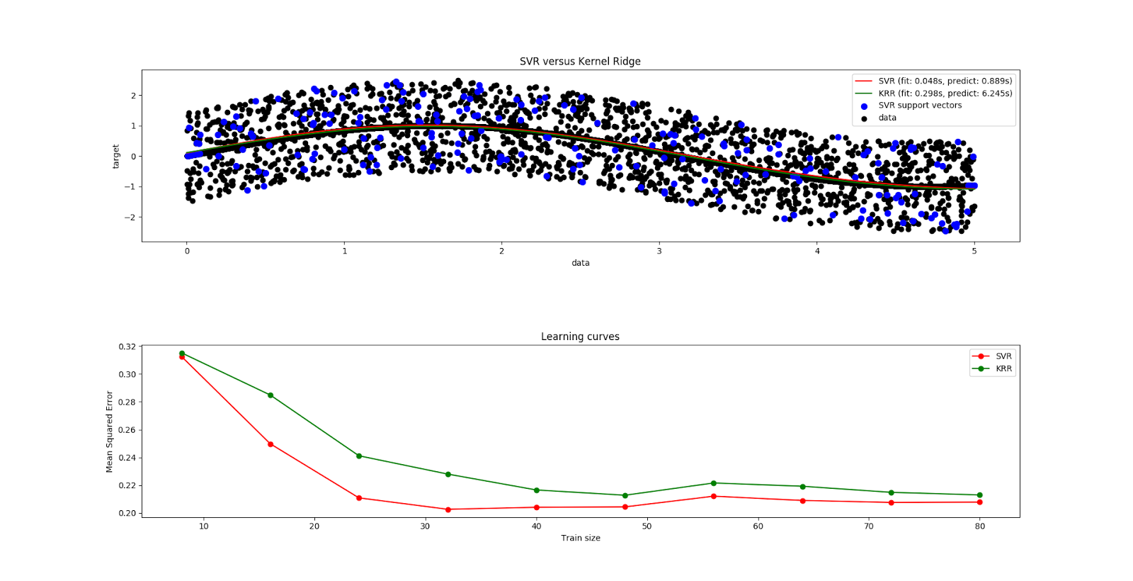
plt.subplot(2,1,1)
# 畫出 SV
plt.scatter(X[sv_ind], y[sv_ind], c='b', s=50, label='SVR support vectors', zorder=2)
# 畫出 data
plt.scatter(X[:], y[:], c='k', label='data', zorder=1)
# 畫出 SVR 的曲線
plt.plot(X_plot, y_svr, c='r',
         label='SVR (fit: %.3fs, predict: %.3fs)' % (svr_fit, svr_predict))
# 畫出 KRR 的曲線
plt.plot(X_plot, y_krr, c='g',
         label='KRR (fit: %.3fs, predict: %.3fs)' % (krr_fit, krr_predict))
plt.xlabel('data')
plt.ylabel('target')
plt.title('SVR versus Kernel Ridge')
plt.legend()
 
# Visualize learning curves
plt.subplot(2,1,2)
 
# model
svr = SVR(kernel='rbf', C=1e1, gamma=0.1, epsilon=0.1)
krr = KernelRidge(kernel='rbf', alpha=0.1, gamma=0.1)
 
# cv = cross-validation，5 表示五份
train_sizes, train_scores_svr, test_scores_svr = \
    learning_curve(svr, X[:100], y[:100], train_sizes=np.linspace(0.1, 1, 10),
                   scoring="neg_mean_squared_error", cv=5)
train_sizes_abs, train_scores_krr, test_scores_krr = \
    learning_curve(krr, X[:100], y[:100], train_sizes=np.linspace(0.1, 1, 10),
                   scoring="neg_mean_squared_error", cv=5)
 
plt.plot(train_sizes, -test_scores_svr.mean(1), 'o-', color="r",
         label="SVR")
plt.plot(train_sizes, -test_scores_krr.mean(1), 'o-', color="g",
         label="KRR")
plt.xlabel("Train size")
plt.ylabel("Mean Squared Error")
plt.title('Learning curves')
plt.legend(loc="best")
 
# 調整之間的空白高度
plt.subplots_adjust(hspace=0.6)
plt.show()

參考

sklearn.kernel_ridge.KernelRidge
sklearn.svm.SVR
sklearn.model_selection.learning_curve